This document aims to introduce the principles, considerations, and common issues of memory management in QuecPython, guiding users in utilizing memory-related features in QuecPython.

Overview

Memory refers to the storage space used by a program during its execution, which stores the instructions and data of the running program, and the stored content changes in real-time. The memory uses RAM (random access memory) as the storage medium, which can read and write data, and the stored data will be lost after power-off. Memory management is an important part of embedded processing systems, mainly responsible for efficient allocation and utilization of memory resources. Due to the limited storage capacity of memory and the dynamic nature of the stored content, a time-division multiplexing strategy can be adopted to meet the space utilization requirements.

Physical Memory Size of Each Platform

Platform	Memory Size
ECx00U & EGx00U series	16MB
EC800GCNGA	16MB
ECx00GCNLD & ECx00GCNLB series	8MB
ECx00N & EGxxxN series	16MB
ECx00MCNLA & ECx00MCNLE & EG810M series	8MB
ECx00MCNLC & ECx00MCNLF & ECx00MCNCC series	4MB
xC200A series	32MB
ECx00E series	1.25MB
BG95 & BG600L series	32MB

QuecPython Memory Management Mechanism

Based on the usage of data in the running program, the memory space can be divided into static storage space and dynamic storage space. Memory management is targeted at dynamic storage space. The distribution of the entire memory is as follows:

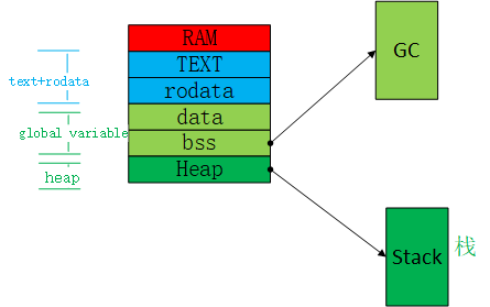
The code segment and constant data belong to the read-only space. Global variables belong to the static storage space. The heap belongs to the dynamic storage space. The GC memory allocated from global variables also belongs to the dynamic storage space. The stack space allocated from the heap also belongs to the dynamic storage space.

Static Memory

Overview

Static storage space refers to the data whose location or address in memory is fixed and unchanged. It includes global variables and static variables, which refer to variable types at the C language development layer.

Global Variables

Global variables are variables with global access attributes, which can be accessed by all functions in the program. They can be divided into uninitialized and initialized variables. The difference between the two is that initialized variables require a copy of the same data to be stored in non-volatile storage such as ROM or flash. Because the data in memory will be lost after power-off, initialized data needs to be preserved after each power failure and restart, so a copy needs to be stored in non-volatile storage.

Static Variables

Static variables are variables defined with the "static" keyword. The GC-managed memory block belongs to this type of space.

Dynamic Memory

Overview

Dynamic storage space refers to the data whose location or address in memory is variable. It includes data allocated in the heap and stack space, which refers to the heap and stack at the C language development layer.

Stack

The stack space is used to store local variables and parameters of functions. The specific allocation and release of stack space are automatically controlled by the system after being given, and developers cannot control it. Each thread will be assigned a different stack space, and the resources will be released when the thread is deleted. The thread stack space is also allocated from the heap space. From the perspective of data structure, the stack space is just an application of the last-in-first-out data structure. Function calls and exits are more in line with the characteristics of this data structure. The allocation and release efficiency is relatively high, suitable for system use.

Heap

The heap is a large memory space allocated and released by developers. Developers have control over it. From the perspective of data structure, it is generally managed in the form of linked lists, which can be randomly accessed and are more flexible, suitable for developers to use.

RTOS Memory Management Algorithms

Overview

Here, memory management only applies to the heap memory space. After the module is powered on and running, a large memory space is reserved as the heap memory. The size of this heap memory space will dynamically change with the start and stop of the application program. Different types of RTOS have different memory management mechanisms. The current module mainly uses two types of RTOS: ThreadX and FreeRTOS.

Common Algorithms

First Fit

First Fit requires that the free partition list be connected in ascending order of addresses. When allocating memory, it starts searching from the first free partition in the list and allocates the first free partition that can satisfy the requirements to the process.

Next Fit

Next Fit is an evolution of the First Fit algorithm. When allocating memory, it starts searching from the next free partition after the last allocated free partition until it finds a free partition that can satisfy the requirements.

Best Fit

Find the smallest free partition that can satisfy the requirements from all free partitions. To speed up the search, the Best Fit algorithm links all free partitions in ascending order of their sizes, so the first found memory that satisfies the size requirement must be the smallest free partition.

Worst Fit

Find the largest free partition that can satisfy the requirements from all free partitions. The Worst Fit algorithm links all free partitions in descending order of their sizes.

Two Level Segregated Fit (TLSF)

Use two-level linked lists to manage free memory, classify free partitions based on their sizes, and use a free list to represent each class of free partitions. The free list index manages these free lists, and each entry corresponds to a free list and records the head pointer of that free list.

Buddy Systems

A variation of the Segregated Fit algorithm, which has better efficiency in memory splitting and merging. There are many types of buddy systems, such as Binary Buddies and Fibonacci Buddies. Binary Buddies is the simplest and most popular one, which classifies all free partitions based on their sizes and uses a free doubly linked list to represent each class. In Binary Buddies, all memory partitions are powers of 2.

Memory Algorithm	Advantages	Disadvantages
First Fit	Large free blocks at high addresses are preserved	Low addresses are constantly fragmented, causing fragmentation; each search starts from the first free partition, increasing the system overhead
Next Fit	Distribution of free partitions is relatively even, low algorithm overhead	Lack of large free memory blocks
Best Fit	Use the smallest memory to meet the requirements and reserve large free memory blocks	The remaining free memory after each allocation is always the smallest, causing many small fragments and high algorithm overhead
Worst Fit	The remaining free memory after each allocation is still large, reducing fragmentation	Lack of large free memory blocks, high algorithm overhead
TLSF	High search efficiency, low time complexity, good performance in fragmentation problems	Complex algorithm and high system overhead during memory recovery
Buddy systems	Severe internal fragmentation	Less external fragmentation

threadx

Allocation

Memory allocation uses the first-fit algorithm, starting from the first free memory block and searching until a suitable size of memory is found.

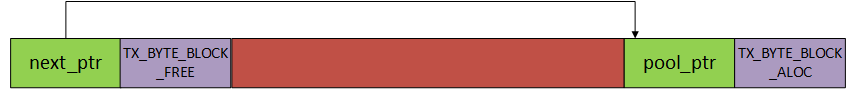
The memory blocks are managed in a linked list manner, with addresses arranged from low to high. The specific linking method is that the first 8 bytes of each memory block are control fields. The first 4 bytes store the starting address of the next memory block, and the next 4 bytes store a specific value, TX_BYTE_BLOCK_FREE, if it is a free memory block, or the starting address of the memory pool management structure if it is an allocated memory block.

During initialization, the entire memory space is divided into two blocks, the first block and the last block. The first 4 bytes of the first block store the starting address of the last block, and the next four bytes are set to TX_BYTE_BLOCK_FREE because they have not been used yet, indicating that it is a free block. The first 4 bytes of the last block store the starting address of the memory pool management structure, and the next 4 bytes are marked as TX_BYTE_BLOCK_ALOC, indicating that it is the last block.

The following figure shows the initial first block of memory being divided into two blocks, the first block and the second block, after the first memory allocation. The first block is returned to the application, and the memory_ptr, which is the starting address of the allocated memory, skips the first 8 bytes because they are control fields and points to the allocated address. The first 4 bytes of the first block store the starting address of the second block of memory, and the next 4 bytes point to the memory pool management structure, indicating that the first block of memory has been allocated and is no longer free memory. The first 4 bytes of the second block of memory point to the third block of memory (the last block of memory), continuing to form a unidirectional linked list. The next 4 bytes store TX_BYTE_BLOCK_FREE, indicating that it is still a free memory block.

Deallocation

During memory deallocation, the control field starting address of the memory block is calculated by subtracting 8 from the deallocated memory's starting address. The starting address of the memory pool management structure is obtained by the first four bytes, and memory deallocation can be performed. After deallocation, the 4th to 8th bytes store TX_BYTE_BLOCK_FREE, indicating that it is a free memory block.

At this time, if the memory is contiguous, no merging or memory rearrangement will be performed. When requesting memory, if the requested size is larger than the current block size, the next block is searched. If it is found that the current block and the next block of memory are contiguous, the current and next blocks are merged into one block.

After memory deallocation, the suspended thread list is checked to see if there are any threads. If there are, an attempt is made to allocate memory and resume thread execution. Thread resumption is done in FIFO order, not in order of thread priority. However, you can call t_byte_pool_prioritize before releasing the thread to move the highest priority thread to the front of the suspended thread list, so that the highest priority thread is resumed first.

Fragmentation Handling

After multiple memory allocations and deallocations, there may be a large number of small memory blocks, which is called memory fragmentation.

When allocating a larger memory, it may be necessary to traverse a large number of small memories, which increases the search overhead and reduces the performance of the algorithm. Since each memory block occupies 8 bytes of control fields, a large number of small memories will result in memory waste. During the search process, if it is found that two neighboring memory blocks are contiguous, the two memory blocks are merged into one block, which is called memory rearrangement.
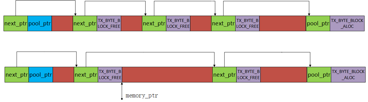
The following figure shows the structure after multiple memory allocations and deallocations. The first block is allocated, and the second, third, and fourth blocks are free memory blocks. The second block has a size of 64 bytes, the third block has a size of 64 bytes, and the fourth block has a size of 256 bytes. Suppose now a memory of size 128 bytes is requested. During the allocation search process, it is found that the second block is too small to meet the requirements, but the second and third blocks are contiguous, so the second and third blocks are merged, and it is found that the merged block exactly meets the request and is returned to the application, as shown in the second figure below.

freertos

FreeRTOS provides 5 memory allocation methods, and FreeRTOS users can choose one of them or use their own memory allocation method. These 5 methods correspond to 5 files in the FreeRTOS source code, namely heap_1.c, heap_2.c, heap_3.c, heap_4.c, and heap_5.c. Each method is suitable for the following scenarios:

Method	Suitable Scenarios
heap_1	Supports memory allocation but not deallocation. Suitable for small embedded devices where memory is allocated at system startup and generally not released during the program's lifetime.
heap_2	Supports memory deallocation but does not merge fragments. Uses the best-fit algorithm. Suitable for scenarios where the size of each memory allocation is relatively fixed.
heap_3	Adds thread safety to the standard library's malloc and free interfaces.
heap_4	Supports memory allocation, memory deallocation, and merging of fragments. Suitable for scenarios where memory is frequently allocated and deallocated with uncertain sizes.
heap_5	Supports multiple non-contiguous regions to form a heap. Suitable for embedded devices with non-contiguous memory distribution.

The module uses the heap_4 method, and here we mainly introduce the algorithm implementation of heap_4.

Allocation

Memory allocation uses the first-fit algorithm, which starts searching for free memory blocks from the beginning and returns the first block that is large enough.

The free memory is maintained through a linked list. The linked list node is defined as follows:

typedef struct A_BLOCK_LINK
{
    struct A_BLOCK_LINK *pxNextFreeBlock;
    /*<< The next free block in the list. */
    size_t xBlockSize;
    /*<< The size of the free block. */
} BlockLink_t;

The two variables are a pointer to the next memory block, pxNextFreeBlock, and the size of the block, xBlockSize. When allocating memory, the system adds heapSTRUCT_SIZE (the size of the linked list node) to the requested size, xWantedSize, to determine the final size to be allocated. Then, it traverses the linked list of free memory starting from the head to find a suitable block of memory. It also checks if there is any remaining memory in the current block (larger than the requested size). If there is, it creates a new node for the remaining memory and inserts it into the free memory list for future allocations. The overall algorithm is similar to the one used in ThreadX.

Deallocation

When deallocating memory, the corresponding linked list node is retrieved by indexing backwards from the memory address. The information of the block is then passed to the linked list insertion function to return the node.

Fragmentation Handling

As seen from the allocation process described above, memory fragmentation can occur after multiple allocations and deallocations. It is necessary to merge these memory fragments into larger blocks. To handle fragmentation, the algorithm is similar to the one used in ThreadX. The free memory list is stored in order of memory address. For example, when inserting a memory block P, the system searches for the memory block A with an address preceding P and checks if there are any allocated blocks between A and P. If not, the blocks are merged. Then, the algorithm checks the position of the memory block C with an address following P. If there are no allocated blocks between P and C, they are merged as well.

Use Cases

Underlying Dynamic Memory Allocation and Deallocation

During the execution of underlying programs, memory space is needed to store data. The malloc interface is called to allocate a certain size of memory from the heap. When the data is no longer needed, the free interface is called to deallocate the memory and return it to the heap.

Thread Creation

When creating new threads during program execution, stack space needs to be allocated for each thread. This stack space is also allocated from the heap. When a thread is deleted after execution, the stack space is deallocated and returned to the heap. Both underlying and application-level programs may create threads.

Common Issues:

How to Avoid Memory Fragmentation

Memory management algorithms can help reduce memory fragmentation, but it cannot be completely avoided. It is recommended to minimize the use of dynamic memory allocation functions and use stack space whenever possible. Allocating and deallocating memory should be done in the same function. It is also advisable to allocate larger chunks of memory at once instead of repeatedly allocating small amounts of memory to reduce memory fragmentation. Designing a memory pool can also help manage memory fragmentation.

Heap Safety Margin

Although heap space is dynamically allocated and deallocated, it is important to ensure that there is enough remaining heap space to meet the memory requirements of complex operations. The total heap space is determined by the underlying system, and this value is fixed after firmware generation. The function _thread.get_heap_size can be used to check the current remaining heap space. For more information on how to use this function, refer to the thread- Multi-threading.

Memory Leaks

Common scenarios for memory leaks include:

• Mismatched memory allocation and deallocation operations, where memory allocated at the beginning of a task is not deallocated when the task ends. This can lead to a continuous decrease in available memory and eventually cause the entire memory to be exhausted, resulting in a program crash.
• Repeated thread creation, where threads are created and deleted without proper pairing. This can lead to the creation of multiple threads for the same task, and each thread requires stack space allocated from the heap. Eventually, this can deplete the entire heap space.

Memory Out-of-Bounds

Common scenarios for memory out-of-bounds include:

• Array out-of-bounds, where the index used to access an array exceeds the actual allocated size, resulting in accessing other memory areas. This can lead to data corruption in other memory areas and cause system program exceptions.
• Stack overflow, where the stack space allocated for a thread is smaller than the actual space required during task execution. This can result in accessing other memory areas during task execution, leading to data corruption in other memory areas and causing system program exceptions.

Memory Allocation Failure Exception Information

Memory allocation failure at the underlying typically triggers a system crash exception.

Application-Level GC Memory

Overview

GC (Garbage Collection) is a memory management mechanism used in Python programming to automatically manage memory. It frees programmers from manually managing memory by identifying and releasing unused resources in memory.

Use Cases

The data allocated in the GC space includes variables from the C language development layer and variables from the Python language development layer.

Management Algorithms

Common Algorithms

Common garbage collection mechanisms include reference counting, mark and sweep, and generational garbage collection.

Reference Counting

The reference counting algorithm works by maintaining an ob_ref field for each object, which records the current number of references to the object. Whenever a new reference points to the object, its reference count, ob_ref, is incremented by 1. Whenever a reference to the object becomes invalid, the reference count is decremented by 1. When the reference count of an object reaches 0, the object is immediately reclaimed, and the memory occupied by the object is freed. The following situations can cause an increment (+1) in the reference count: object creation, object being referenced, object being passed as a parameter to a function, and object being stored as an element in a container. The following situations can cause a decrement (-1) in the reference count: explicit destruction of object aliases, assignment of new objects to object aliases, and objects leaving their scope (e.g., when a function finishes execution and local variables are destroyed or when an object is removed from a container).

The reference counting algorithm has the disadvantage of requiring additional space to maintain reference counts and cannot handle the problem of "circular references" where objects reference each other and their reference counts never reach 0, preventing their reclamation.

a = [1, 2]  # reference count is 1
b = [2, 3]  # reference count is 1
a.append(b)  # reference count is 2
b.append(a)  # reference count is 2
del a  # reference count is 1
del b  # reference count is 1

Mark and Sweep

The mark and sweep algorithm consists of two phases: the mark phase and the sweep phase. In the mark phase, all objects are traversed, and if an object is still referenced, it is marked as reachable. In the sweep phase, all objects are traversed again, and if an object is not marked as reachable, it is reclaimed.

Objects are connected through references (pointers), forming a directed graph, where objects are nodes and reference relationships are edges. Starting from the root object, objects are traversed along the edges, and reachable objects are marked as active objects. Unreachable objects are non-active objects that need to be cleared. Root objects are some global variables, call stacks, and registers; these objects cannot be deleted.

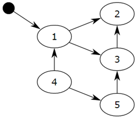
Starting from the small black circle, object 1 is reachable, so it will be marked. Objects 2 and 3 are indirectly reachable and will also be marked, while 4 and 5 are not reachable. Therefore, 1, 2, and 3 are active objects, while 4 and 5 are inactive objects that will be garbage collected.

Generational Collection

The principle of generational collection algorithm is based on the statistical fact that for a program, there is a certain proportion of memory blocks with short lifetimes, while the remaining memory blocks have longer lifetimes, even lasting from the beginning to the end of the program. The proportion of short-lived objects is usually between 80% and 90%. Therefore, the longer an object exists, the less likely it is garbage and the fewer objects need to be traversed during garbage collection, thus improving the speed of garbage collection.

The specific method is to divide all objects into three generations: 0, 1, and 2. All newly created objects are generation 0 objects. If an object in a certain generation survives garbage collection, it will be moved to the next generation. Each generation can have a threshold, for example, triggering a generation 0 garbage collection every 101 newly allocated objects. Every 11 generation 0 garbage collections trigger a generation 1 garbage collection. Every 11 generation 1 garbage collections trigger a generation 2 garbage collection. Before executing garbage collection for a certain generation, the objects in the young generation object list are also moved to that generation for garbage collection. An object is gradually moved to the old generation over time, and the frequency of garbage collection decreases.

QuecPython Management Mechanism

QuecPython uses a mark-and-sweep mechanism to manage memory.

Initialization

In QuecPython, the smallest unit of memory is a block, and the size of each block is defined by the macro MICROPY_BYTES_PER_GC_BLOCK, which is 16 bytes in our code. At least one block will be allocated each time. Each memory block has four possible states:

• FREE(free block): Indicates that the block is unused, represented by the value 0x0.

• HEAD(head of a chain of blocks): Indicates that the block is allocated and is the first block of a chain of allocated blocks, represented by the value 0x1.

• TAIL(in the tail of a chain of blocks): Indicates that the block is allocated and is not the first block of a chain of allocated blocks, represented by the value 0x2.

• MARK(marked head block): Indicates that the block is marked as referenced during memory collection and should not be released, represented by the value 0x3.

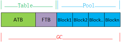
The status flags of these memory blocks are stored in a separate block of memory called ATB (Allocation Table Byte), located at the beginning of the GC memory. Since 2 bits can represent 4 states, one byte can record the usage status of 4 memory blocks. The size of ATB is proportional to the total size of GC memory.

In addition to the status flags mentioned above, each memory block also has a finalizer flag, indicating whether the block is a finalizer memory or not, represented by the values 0 and 1. The finalizer flags are stored in a separate block of memory called FTB (Finalizer Table Byte), located after the ATB space. Since 1 bit can represent this status, one byte can mark the finalizer status of 8 memory blocks. The size of FTB is also proportional to the total size of GC memory. The finalizer flag is not directly related to memory allocation and collection, but is used to distinguish the internal mechanism's choice. (The purpose of the finalizer flag: It is used internally. When an object is instantiated using m_new_obj_with_finalizer for memory allocation, the memory allocation is marked as a finalizer. When the memory is collected, if the memory is marked as a finalizer and the object structure's first member is mp_obj_base_t base, the delete method of this object will be automatically found and executed before releasing the memory. Use case: When the virtual machine restarts, all resources will be reclaimed, so the callback function information passed down from the Python layer to the C layer will become invalid. If the C layer uses these resources again, an exception will be triggered. In this case, the delete method of the object can be called during GC memory collection to deinitialize the underlying resources and clear the callback function information.)

The initialization of GC memory is implemented by the gc_init function. First, a large static memory space is allocated as the total available memory space for GC. Then, the entire GC memory is divided into three parts:

• ATB (Allocation Table Byte): A continuous memory starting from the beginning of the GC memory, used to mark the usage status of dynamically allocated and released memory blocks.

• FTB (Finalizer Table Byte): A continuous memory immediately following the ATB memory, used to mark whether a memory block is a finalizer type.

• P (Pool): A memory pool used for dynamic allocation and release, with the address range from after the ATB and FTB memories to the end of the GC memory. The minimum allocation unit is a block, 16 bytes.

The distribution of GC memory is shown in the following diagram:

Allocation

We use the m_new_xxx interface to allocate GC memory, which ultimately calls the gc_alloc function to allocate memory.

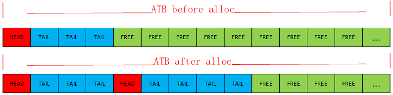
The allocation process is as follows: First, the size (in bytes) of the memory to be allocated is converted to the number of blocks, n_blocks. Then, the GC memory is searched for a contiguous segment of n_blocks free memory. If a segment of the required size is found, the ATB position corresponding to the first block of that segment is marked as HEAD (0x1), and the ATB positions corresponding to the second to last blocks of that segment are marked as TAIL (0x2). If the memory is allocated using m_new_obj_with_finalizer, it means that the segment of memory is of the finalizer type, and the FTB position corresponding to the first block of that segment is marked as finalizer (0x1). Finally, the physical address corresponding to the first block of that segment is returned to the user.

The process of finding a suitable memory block: In general, each time the search starts from the beginning of ATB, and if a free block is found, the counter n_free is incremented by 1. If a non-free block is encountered during the search, the counter is reset to 0 and the search starts again. This process continues until n_free is greater than or equal to the number of memory blocks n_blocks to be allocated. In the case where n_blocks is 1, the ATB position corresponding to the found free block is used as the starting address for the next memory allocation search. Because all blocks before that position are definitely not free, there is no need to start the search from the beginning next time. However, after each memory collection, the starting address for the search is reset to the beginning of ATB.

From the above process, this allocation method is similar to the first-fit algorithm. As the number of allocations increases, there may be a continuous splitting of existing large memory blocks, resulting in memory fragmentation.

The content distribution of ATB before and after one allocation is shown in the following diagram.

Collection

If there is insufficient memory during GC memory allocation, the gc_collect function is triggered for memory collection. Memory collection mainly consists of two steps:

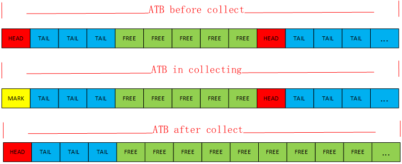
Step 1: Scan all Python threads and the global information recorded in the mp_state_ctx structure. This scan action finds the global information recorded in mp_state_ctx and all addresses appearing in the thread stack that are within the range of GC memory. If the ATB flag corresponding to the block where the address is located is HEAD (0x1), it means that the memory is still in use, so the ATB flag is changed from HEAD (0x1) to MARK (0x3).

Step 2: Scan the entire GC memory for ATB flags. In this step, all blocks that are in the HEAD (0x1) state and the blocks following them that are marked as TAIL (0x2) are marked as FREE (0x0). This is because in the previous scanning step, these blocks were not marked as MARK (0x3), indicating that they are no longer in use. This way, this segment of memory is reclaimed. Additionally, all blocks that are in the MARK (0x3) state are changed to HEAD (0x1), restoring them to normal usage. After these two steps, the GC memory collection is complete.

The distribution of ATB content before and after the collection is shown in the following diagram:

Fragmentation Handling

From the memory reclamation process described above, contiguous free blocks are automatically merged after collection, allowing them to be allocated together in the next memory allocation.

Frequently Asked Questions

How to configure the GC collection threshold?

Use the gc.threshold() function to set the collection threshold, which is measured in bytes. When the accumulated allocated memory size exceeds this threshold, the GC memory collection will be triggered.

How to check the remaining GC memory?

Use micropython.mem_info(). This interface is not yet available and will be made available in the latest firmware version. An example of executing this function is as follows:

>>> import micropython
>>> micropython.mem_info()
stack: 884
GC: total: 320128, used: 13136, free: 306992
 No. of 1-blocks: 228, 2-blocks: 61, max blk sz: 264, max free sz: 19177

In the output, total represents the total size of the GC memory space in bytes, used represents the currently allocated GC memory size in bytes, and free represents the remaining available GC memory size in bytes. No. of 1-blocks represents the number of GC memory blocks allocated with a size of 1 block (16 bytes), and 2-blocks represents the number of GC memory blocks allocated with a size of 2 blocks (2x16 bytes). max blk sz represents the size of the largest block in the currently allocated GC memory blocks, measured in blocks (16 bytes per block). max free sz represents the size of the largest block in the remaining available GC memory blocks, measured in blocks (16 bytes per block).

When will the GC collection be triggered?

The GC collection will be triggered in the following situations:

• When the allocated memory size exceeds the set threshold.

• When memory allocation fails.

• When the gc.collect() function is called actively.

How to trigger the GC collection?

Call the gc.collect() function. For specific usage of this function, refer to the gc- Control the Garbage Collector.

Python Programming Considerations

Stack Overflow, Thread Stack Too Small

If the stack space size is smaller than what is required by the business logic, it may cause data operations during the business process to go beyond the boundaries of other memory spaces, leading to data corruption and system program exceptions. Therefore, it is necessary to allocate an appropriate stack space size based on the complexity of the business logic. This can be done by calling the _thread.stack_size() function before creating a thread. For specific usage of this function, refer to the thread- Multi-threading.

Using Variables After They Have Been Garbage Collected

Variables Allocated by the Python Virtual Machine

The underlying system ensures that variables in use can be marked, that is, the reference graph is reachable.

User-defined Variables in Python

Python has the following scopes:

• L (Local) - Local scope
• E (Enclosing) - Functions outside of a closure function
• G (Global) - Global scope
• B (Built-in) - Built-in scope

Objects that need to be in the global scope must be defined as global objects. At the same time, ensure that objects in the local scope are not relied upon by global scope business logic. This is because during GC memory collection, local scope objects that have finished executing will be released. If the business logic still relies on these objects, it may cause certain functions to fail.

Considerations and examples for proper usage:

• If a local scope object is created and a callback function is registered with the underlying system, and then the local object is garbage collected during GC memory collection, the callback may not be triggered and the functionality may be lost. The following is an example of using the power key, where a callback function is registered.

Incorrect example:

from misc import PowerKey
import utime

def callback(info):
    global start_time, end_time
    if info == 1:
        start_time = utime.time()
    else:
        end_time = utime.time()
        if end_time - start_time >= 3:
            print('long press')
        else:
            print('short press')

def run():
    PowerKey().powerKeyEventRegister(callback) # The PowerKey object will be garbage collected after GC memory collection, causing the registered callback function to lose functionality

run()

Correct example:

from misc import PowerKey
import utime

def callback(info):
    global start_time, end_time
    if info == 1:
        start_time = utime.time()
    else:
        end_time = utime.time()
        if end_time - start_time >= 3:
            print('long press')
        else:
            print('short press')

global pwk
pwk = PowerKey() # The PowerKey object is stored in the global object pwk, so it will still be available after GC memory collection and the registered callback function will continue to work
pwk.powerKeyEventRegister(callback)

GC Memory Allocation Failure

Possible Causes

• Insufficient total space.

• Memory fragmentation.

How to Avoid

Insufficient Total Space

Consider whether there are unnecessary global objects in the Python code and convert them to local objects.

Memory Fragmentation

Set the GC collection threshold to 75% of the total memory space. This means that whenever the accumulated allocated GC memory size exceeds 75% of the total memory, a collection will be triggered. This ensures that there is a portion of large contiguous free memory space. Additionally, it is important to note that the list.append() operation actually requests a large contiguous block of memory. As the list continues to expand, it may fail to obtain a contiguous block of large memory space and return an error.

System Time

Data Formatting